An OpenFE RBFE campaign in your own AWS: a TYK2 walkthrough
A full OpenFE relative binding free-energy campaign — 10 TYK2 ligands, a 9-edge network — planned, fanned out across A10G spot GPUs, and gathered into a ΔΔG table in line with published results, as one managed Slurm campaign in your own AWS account. Single-replicate run, scoped honestly below.
Published June 2 2026. Numbers are from a single end-to-end run (job 2958, June 1–2 2026) on Clusterra's dev cluster: OpenFE 1.11.1, 5 ns production / 1 ns equilibration / 11 λ-windows, single replicate (n=1), on a 9-edge minimal-spanning network. Experimental reference values are the canonical TYK2 set from
OpenFreeEnergy/openfe-benchmarks(cross-checked against the OpenFFprotein-ligand-benchmarkKi data; primary measurements: EJMECH 10.1016/j.ejmech.2013.03.070, JMC 10.1021/jm400266t). This validates the managed pipeline and the operating model — not generalization to novel chemistry, and not an accuracy claim. TYK2 is the easy, well-trodden benchmark; a single replicate yields per-edge ΔΔG only (no ranking plot, no error bars), and a 9-point comparison cannot distinguish between methods. The n=3 production reproduction is the gate for any accuracy statement; see Honest scope.
Running an OpenFE RBFE campaign in your own AWS
Ten TYK2 ligands in, a ΔΔG table out — a 9-edge perturbation network run as 18 alchemical edge-legs at 5 ns/window, planned, fanned out across A10G spot GPUs, recovered through spot reclaims, and gathered, all as one managed Slurm campaign inside the customer's own AWS account.
The thing being demonstrated here is the operating model, not a number: a lone computational chemist runs a production-length FEP campaign on open tools they control (OpenFE, OpenMM), in their own cloud account, without standing up an HPC cluster, babysitting spot evictions, or hand-managing 18 GPU jobs — and the whole run (network plan, per-edge ΔΔG, cost, provenance) lands as one queryable record in their account. The accuracy numbers check out — they sit within experimental noise of published OpenFE and FEP+ TYK2 results — but at n=1 on 9 edges they are a sanity check that the pipeline is wired correctly, not a benchmark claim. We are explicit about that throughout.
TL;DR (n=1, June 1–2 2026)
- 3 templates, 1 campaign.
openfe-plan-network(plan the network) →openfe-rbfe-run(Slurm array, one task per edge-leg,--resumefor spot) →openfe-gather(collect ΔΔG). Open licenses end-to-end. - The operating model: one Slurm array fanned out 18 single-GPU jobs across A10G spot; several legs were reclaimed mid-run and resumed from checkpoint with zero lost work; the scientist never touched a cluster. One campaign, one provenance trail, in the customer's own AWS account.
- System: TYK2, 10 ligands from the canonical JACS/EJMECH+JMC series, OpenFE
rbfe_tutorialstructures; minimal spanning tree → 9 edges → 18 edge-legs (complex + solvent per edge). - Protocol: OpenFE 1.11.1, OpenMM Hamiltonian replica exchange, 11 λ-windows, 1 ns equilibration + 5 ns production, OpenFF Sage 2.2.1 + ff14SB + TIP3P, AM1-BCC charges. Single replicate. (Full settings in the appendix.)
- Accuracy (per-edge ΔΔG, 9 edges) — a sanity check, not a benchmark: MUE 0.38 kcal/mol (95% CI [0.23, 0.55]), RMSE 0.46 [0.27, 0.61], Pearson R 0.85 [−0.29, 0.98]. On the same TYK2 set, published per-edge references are FEP+ 0.75 / 0.93 / 0.89 (Wang 2015) and open-source OpenFE 0.75 / 0.94 (n=1). With 9 points and ~0.4 kcal/mol experimental error, these are statistically indistinguishable — parity within noise, not an improvement.
- Cost: ~$33 of the customer's own AWS spot for the full 9-edge campaign (~$3.7 per edge; an edge = its complex + solvent leg).
- Hardware reality (measured): complex legs peak at ~3.7–4.5 GB VRAM at 95–100% GPU utilization; solvent legs ~0.5 GB. The A10G's compute is saturated; only its 24 GB VRAM is over-provisioned.
Setup
Target. TYK2 (JAK-family kinase), the canonical RBFE benchmark — well-behaved congeneric transformations, published experimental affinities, a known convergence profile. Deliberately the easy benchmark: the right fixture for checking that the managed pipeline produces correct numbers, not for claiming accuracy on hard targets.
Ligands (10). ejm_31, ejm_42, ejm_43, ejm_46, ejm_47, ejm_48, ejm_50 (EJMECH series, Ki in µM) and jmc_23, jmc_27, jmc_28 (JMC series, Ki in nM, cis enantiomer), from the OpenFE rbfe_tutorial set. We discard the shipped partial charges and regenerate AM1-BCC at plan time (AmberTools) for one consistent charge model across the network.
Network. openfe plan-rbfe-network, Kartograf atom mapper (OpenFE 1.11 default), minimal spanning network over LOMAP scores → 9 edges connecting the 10 ligands, emitted as 18 transformation JSONs (complex + solvent leg per edge). Each JSON is a self-contained alchemical transformation openfe quickrun executes independently — the unit of Slurm fan-out. Note: a minimal spanning tree selects the highest-similarity (easiest) perturbations and contains no cycles — see the caveats this carries in Honest scope.
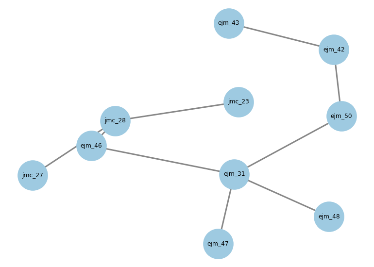
The TYK2 perturbation network: 10 ligands (nodes) connected by 9 alchemical transformations (edges) as a minimal spanning tree, with ejm_31 as the hub. Each edge becomes one openfe-rbfe-run array task (a complex + a solvent leg). The tree structure is visible — and so is the absence of cycles, which is why this run carries no cycle-closure check.
Results — a sanity check, read with the caveats
Per-edge ΔΔG vs experiment
| Edge | ΔΔG calc (kcal/mol) | ΔΔG exp (kcal/mol) | error |
|---|---|---|---|
| ejm_31 → ejm_46 | −1.0 | −1.77 | +0.77 |
| ejm_31 → ejm_47 | +0.1 | −0.16 | +0.26 |
| ejm_31 → ejm_48 | +0.8 | +0.54 | +0.26 |
| ejm_31 → ejm_50 | +0.2 | +0.56 | −0.36 |
| ejm_42 → ejm_43 | +1.4 | +1.52 | −0.12 |
| ejm_42 → ejm_50 | −0.0 | +0.80 | −0.80 |
| ejm_46 → jmc_28 | +0.3 | +0.33 | −0.03 |
| jmc_23 → jmc_28 | +0.4 | +0.72 | −0.32 |
| jmc_27 → jmc_28 | +0.8 | +0.30 | +0.50 |
(Experimental ΔΔG values carry ~0.4 kcal/mol uncertainty; per-edge errors are shown to 0.01 only for arithmetic transparency, not because they're resolved to that precision.)
MUE 0.38 [0.23, 0.55] · RMSE 0.46 [0.27, 0.61] · Pearson R 0.85 [−0.29, 0.98] (n = 9 edges; 95% bootstrap CIs).
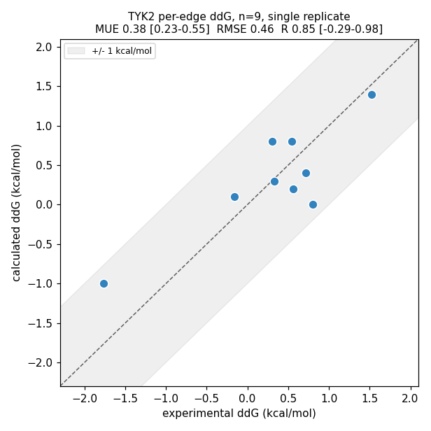
Calculated vs experimental ΔΔG for all 9 edges (single replicate). Every point falls within the ±1 kcal/mol band. The wide bootstrap CIs — R especially, at [−0.29, 0.98] — are precisely why this is a sanity check that the pipeline produces sane numbers, not a benchmark claim.
How that compares — and why we make no accuracy claim
On the same TYK2 set (the one defined by Wang et al., JACS 2015, crystal 4GIH), published per-edge ΔΔG references are:
| Method (TYK2, per-edge ΔΔG) | MUE | RMSE | R | edges · replicate | source |
|---|---|---|---|---|---|
| OpenFE on Clusterra (this run) | 0.38 [0.23–0.55] | 0.46 | 0.85 [−0.29–0.98] | 9 · n=1 | job 2958 |
| Schrödinger FEP+ | 0.75 | 0.93 | 0.89 | 24 · n=1 | Wang 2015, Table 2 (DOI 10.1021/ja512751q) |
| OpenFE (open-source ref) | 0.75 / 0.66 | 0.94 / 0.83 | — | 24 · n=1 / n=5 | Rufa et al. (PMC9333416) |
It is tempting to read our row as "better." It isn't, and we won't claim it is, for three independent reasons:
- Within noise. Experimental error is ~0.4 kcal/mol — about the size of our MUE. With 9 points you cannot statistically distinguish 0.38 from 0.75. The honest statement is parity within noise.
- The R is unconstrained. Pearson R = 0.85 sounds strong, but its 95% bootstrap CI is [−0.29, 0.98] — at n=9 the correlation is essentially undetermined. We report it for completeness, not as evidence.
- Our 9 edges are a favorable subset. A minimal spanning tree picks the easiest (highest-similarity) perturbations, and we ran 24→9 of the canonical set with a different atom-mapping. So our subset is expected to flatter the MUE relative to the references' full 24-edge networks.
We also deliberately do not compare this per-edge ΔΔG against pooled per-ligand ΔG figures (e.g. the OpenFE 2024 industry benchmark's ~1.73 kcal/mol) — that's a different metric.
Per-leg statistical error (MBAR)
gather --report raw per-leg MBAR uncertainties run 0.1–0.5 kcal/mol on complex legs, ~0.1 on solvent legs — real single-replicate statistical error. (The network-level uncertainty column reads 0 because it's the std across replicates, undefined at n=1.)
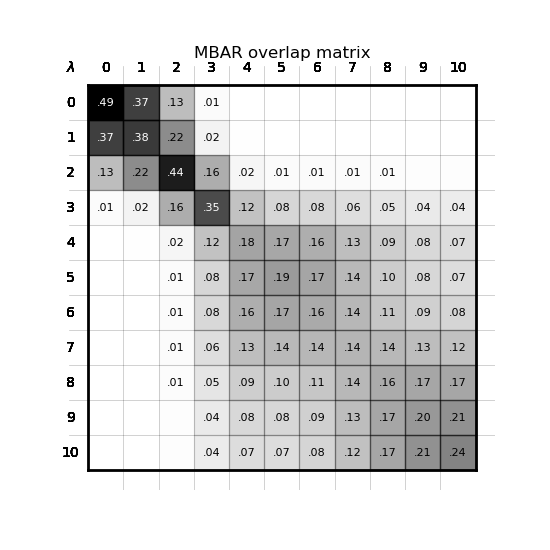
MBAR overlap matrix for one edge's 11 λ-windows (complex leg, ejm_31→ejm_46), produced automatically by openfe quickrun. The band-diagonal structure — non-trivial overlap between adjacent windows — is the per-leg convergence check: evidence the alchemical path was sampled well enough to trust the ΔG, even though a spanning-tree network carries no cycle-closure check at the network level.
The operating model: what you actually get
This is the part that matters for a lone comp chemist, because it's the part they don't have to build.
One Slurm array, 18 single-GPU jobs. RBFE at this scale is embarrassingly parallel — each edge-leg is an independent single-GPU OpenMM run (the 11 λ-windows are replica-exchanged within one GPU). openfe-rbfe-run emits #SBATCH --array=1-18; task N runs the Nth transformation. No multi-node MPI, no gang scheduling.
Spot, with a real safety net — tested by reality. Every leg ran on A10G spot. Several legs were reclaimed mid-run; openfe quickrun --resume reused the cached ProtocolDAG and continued from checkpoint, so those legs' wall times stretched to 4–5 h across interruptions and finished cleanly. Zero lost work. That resilience is wired into the template, not something the scientist configures per run.
Right-sized GPUs, measured not guessed. nvidia-smi sampling on every leg: complex legs peak ~3.7–4.5 GB VRAM at 95–100% GPU utilization; solvent ~0.5 GB. Consequences: (1) the A10G's 24 GB is heavily over-provisioned, so the cheapest A10G instance is the right node — most legs landed on g5.xlarge (~$0.49/hr spot); (2) because the GPU compute is saturated, packing multiple legs per GPU wouldn't help — the headroom is VRAM, not FLOPs.
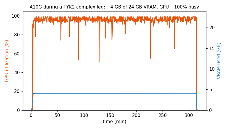
One complex leg, ~5 h on an A10G: GPU utilization (orange) pinned near 100% the entire run, while VRAM (blue) sits flat at ~4 GB of the card's 24 GB. The compute is saturated — so packing more legs onto the GPU wouldn't help — while ~83% of the VRAM goes unused, which is why the smallest A10G instance is the right node, not a bigger card.
"Why not just pip install openfe and run this on my own spot?"
Fair question — OpenFE is free and open, and if you have an HPC engineer and the time, you can. What this campaign did around the science is the actual product:
- The orchestration you didn't write: the network→array fan-out, the spot-reclaim checkpoint-resume, the GPU right-sizing, the per-leg cost stamping, the gather. That's the multi-day plumbing between "OpenFE exists" and "18 legs ran and recovered on spot without me watching."
- Operated end-to-end: the scientist never SSHed into a node, sized an instance, or rescued an evicted job.
- In your own account, as a record: the plan, the ΔΔG table, the costs, and the provenance accrete in your AWS — a queryable campaign history, not scattered job folders. Over many cycles that accreting record is the thing you'd otherwise rebuild by hand.
If you have a platform team, you can build this. The product is for the team that doesn't — and the durable value is the operated, in-account campaign record, not the compute price.
(On MPI, briefly: a 30k-atom RBFE leg is single-GPU by design — OpenMM's CUDA platform doesn't decompose one simulation across GPUs, and openfe quickrun runs single-GPU regardless. MPI is neither needed nor used here.)
Honest scope (what this run is and isn't)
- Single replicate (n=1). Per-edge ΔΔG only. The per-ligand ΔG MLE and the ΔΔG-vs-experiment ranking scatter (the usual FEP "money plot") require ≥2 replicates —
gather --report dgrefuses on n=1 (Every edge must have at least two simulation repeats). No inter-replicate error bars exist. A real accuracy claim requires the n=3 reproduction (roughly 3× this run, ~$70–100 on the same spot). - Favorable, cycle-free network. The minimal spanning tree selects the easiest perturbations and contains no cycles — so there is no cycle-closure (hysteresis) self-consistency check in this run. The n=3 reproduction will use a redundant network for closure QC.
- 9-point statistics. Every headline metric has a wide CI (above); R is effectively undetermined. Treat the numbers as "pipeline produces sane values," not "method is accurate."
- TYK2 is the easy benchmark, with ligands in the lineage these force fields were tuned against. No claim about novel chemistry, charge-changing perturbations, cofactors, or harder targets.
- Reference values are a self-consistent set (openfe-benchmarks / OpenFF trace to the same EJMECH/JMC primary Ki data), with ~0.4 kcal/mol experimental error — comparable to the MUE.
Run it in your own AWS
OpenFE RBFE free-energy campaigns — and the rest of your HPC stack — run on a managed Slurm cluster in your own AWS account: on spot, no cluster to stand up, no data egress. Start at clusterra.cloud, or email hello@clusterra.cloud.
Protocol appendix (for reproduction)
OpenFE 1.11.1 RelativeHybridTopologyProtocol, OpenMM 8.4.0 + openmmtools 0.26.0:
- Sampling: Hamiltonian replica exchange (
repex), 11 λ-windows, 2.5 ps / exchange iteration; 1 ns equilibration + 5 ns production per window; 5000 minimization steps. - Integration: hydrogen-mass repartitioning (H mass 3.0 amu) → 4 fs timestep; HBond constraints; rigid water.
- Force fields: OpenFF Sage 2.2.1 (ligands), AMBER ff14SB (protein), TIP3P water; AM1-BCC ligand charges via AmberTools (regenerated at plan time).
- System: PME electrostatics, 0.9 nm nonbonded cutoff, dodecahedral box, 0.15 M NaCl.
- Platform: CUDA forced explicitly (
OPENMM_DEFAULT_PLATFORM=CUDA) so a mis-provisioned node fails loudly rather than silently dropping to the (orders-of-magnitude slower) CPU platform. - Environment: micromamba on EFS, reused across jobs; CUDA pinned to 12.6 — the default resolve pulls 13.3, whose PTX the host driver (max CUDA 13.2) rejects with
CUDA_ERROR_UNSUPPORTED_PTX_VERSION; a one-linecuda-version=12.6pin fixes it. - Remaining parameters are OpenFE 1.11 defaults; the exact plan JSON for job 2958 reproduces this run verbatim.
Reproduce it
Three templates in the catalog:
openfe-plan-network— ligand SDF + receptor PDB → network + per-edge transformation JSONs + manifest. CPU, minutes.openfe-rbfe-run—#SBATCH --array=1-N, one task per transformation,--resumefor spot. A10G GPU.openfe-gather— results directory → ΔΔG / per-leg TSV.
Point stage 1 at your own prepared receptor and ligand series, set the production length and replicate count, and the same campaign runs in your AWS account on your spot — one Slurm queue, operated end-to-end, the run history living where your data already does.